
Simulation studies were performed to investigate for which conditions of sample size of patients (n) and number of repeated measurements (k) (e.g., raters) the optimal (i.e., balance between precise and efficient) estimations of intraclass correlation coefficients (ICCs) and standard error of measurements (SEMs) can be achieved. Subsequently, we developed an online application that shows the implications for decisions about sample sizes in reliability studies. We simulated scores for repeated measurements of patients, based on different conditions of n, k, the correlation between scores on repeated measurements (r), the variance between patients’ test scores (v), and the presence of systematic differences within k. The performance of the reliability parameters (based on one-way and two-way effects models) was determined by the calculation of bias, mean squared error (MSE), and coverage and width of the confidence intervals (CI). We showed that the gain in precision (i.e., largest change in MSE) of the ICC and SEM parameters diminishes at larger values of n or k. Next, we showed that the correlation and the presence of systematic differences have most influence on the MSE values, the coverage and the CI width. This influence differed between the models. As measurements can be expensive and burdensome for patients and professionals, we recommend to use an efficient design, in terms of the sample size and number of repeated measurements to come to precise ICC and SEM estimates. Utilizing the results, a user-friendly online application is developed to decide upon the optimal design, as ‘one size fits all’ doesn’t hold.
Avoid common mistakes on your manuscript.
In clinical trials conclusions are drawn based on outcome measurement scores. These scores are measured with measurement instruments, such as clinician-reported outcome measures, imaging modalities, laboratory tests, performance-based tests, or patient-reported outcome measures (PROMs) (Walton et al. 2015). The validity (or reliability) of trial conclusions depend, among other things, on the quality of the outcome measurement instruments. High quality measurement instruments are valid, reliable, and responsive to measure the outcome of interest in the specific patient population.
Reliability and measurement error are two related but distinct measurement properties that can be investigated within the same study design (using the same data). Measurement error refers to how close the results of the repeated measurements are. It refers to the absolute deviation of the scores, or the amount of error, of repeated measurements in stable patients (de Vet et al. 2006), and is expressed in the unit of measurement such as the standard error of measurement (SEM) (de Vet et al. 2006; Streiner and Norman 2008). Reliability relates the measurement error to the variation of the population. Therefore, reliability refers to whether and to what extent an instrument is able to distinguish between patients (de Vet et al. 2006). For continuous scores, reliability is expressed as an intraclass correlation coefficient (ICC), a relative parameter.
In a study on reliability, we are interested in the influence of specific sources of variation such as rater, occasion or equipment, on the score (Mokkink et al. 2022). This specific source of variation of interest (e.g., rater) is varied across the repeated measurements in stable patients. For example, we are interested in the influence of different raters (i.e., the source of variation that is varied across the repeated measurements) on one occasion (inter-rater reliability), or in the influence of different occasions (i.e., the source of variation that is varied across the repeated measurements) by one rater on the score of stable patients (i.e., intra-rater reliability); or in the influence of the occasion on the score when stable patients rate themselves on different occasions with a self-administered questionnaire (i.e., test–retest reliability). In the remainder of this paper, the term ‘repeated measurements’ refers to repeated measurements in stable patients, ‘different raters’ will be used as example of the source of variation of interest, and the term ‘patients’ will be used to refer to the ‘subjects of interest’.
Multiple statistical models can be used to estimate ICCs and SEM. Often used models are the one-way random effects model, the two-way random effects model for agreement and the two-way mixed effects model for consistency (see Table 1 and “Appendix 1” for model specifications of ICCs and SEMs). Three-way effects models are outside the scope of this paper. The research question together with the corresponding design of the study determine the appropriate statistical model to analyze the data (Mokkink et al. 2022).
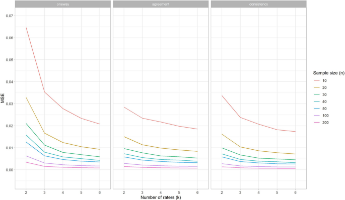
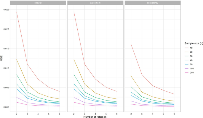
The presence of a systematic difference between raters increased the MSE values for ICCone-way, but not for ICCagreement, and ICCconsistency (see online tool). This means that the required sample size for the one-way effects models increases when a systematic difference between raters occurs, while the required sample sizes for the two-way effects models remains the same.
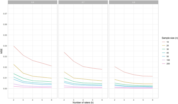
Next, we noticed an influence of the correlation between scores on repeated measurements (r) on the MSE values for all types of ICCs, specifically when no rater deviated (Fig. 2 shows the MSE per correlation condition for ICCagreement). That is, increasing correlation (i.e., 0.8 instead of 0.6) leads to decreasing MSE values. When one rater deviates, r continues to affect the MSE for ICCconsistency to the same extent, but to a lesser extent for ICCagreement and ICCone-way (“Appendix 2”).
Overall the bias for the SEM was very small and thus negligible. All results for bias can be found in the online application.
In Fig. 3 we plotted the MSE values of the SEMagreement estimations for the number of raters per condition of sample size (shown in different colors), for one rater with a systematic difference and for each of the three conditions of r. Similar as we saw above for the MSE curves for ICCs, the steepness of the curves declines most between k = 2 and k = 3, especially for a sample size up to n = 50. Moreover, we see the distance between the curves decreases when n increases, especially in the curves up to n = 40. The MSE values for condition n = 30 and k = 4 for any of the three conditions r is very similarly compared to the condition n = 50 and k = 3 when r = 0.6, or n = 40 and k = 3 when r is higher.
So, we can conclude that the influence of the correlation r on the MSE value for SEM estimations is similar to the influence of r on the MSE values for ICC estimations.
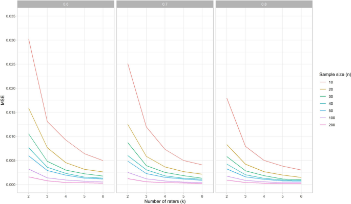
In both SEMone-way and SEMagreement models all measurement error is taken into account (see “Appendix 1”), so the resulting SEM estimates are equal between these models (Mokkink et al. 2022). The MSE values for SEMconsistency are nearly the same if no rater deviates or when one rater deviates. When no rater deviates, the MSE values for the SEMone-way and SEMagreement are only slightly lower compared to the SEMconsistency (data available in the online application). However, aberrant from the MSE results for the ICC estimations (see Fig. 1), the MSE values for the SEMone-way and SEMagreement increase when one of the raters systematically deviates (see Fig. 4).
With no systematic difference between raters the coverage of the 95% confidence intervals around the ICC estimation was as expected, i.e., around the 0.95 for all three types of ICCs. As there were no differences found for the simulation study conditions (i.e., r, v, n and k) the results for coverage are only separated per type of ICC (Fig. 5, left panel).
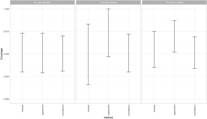
The coverage of the ICCconsistency is very similar when one or two raters deviate, compared to the situation when no rater deviates. However, when one of the raters deviates the lowest coverage of the 95% confidence intervals around the ICCone-way estimation decreases (i.e., under-coverage) and the highest coverage increases (i.e., over-coverage) (Fig. 5, middle panel). While this change in coverage disappears again when two raters deviate (Fig. 5, right panel). Note that in this latter scenario always more than three raters are involved. Furthermore, the ICCagreement showed an over-coverage when one or two raters systematically deviated from the other raters, as the lowest value and the highest value for the coverage of the 95% confidence intervals around the ICCagreement both increase (Fig. 5 middle and right panel). A coverage of 1 means that the ICC of the population always fell within the 95% confidence intervals of the ICC estimation. This was due to the fact that the width of the confidence intervals around these estimations were very large, i.e., confidence interval width around 1.
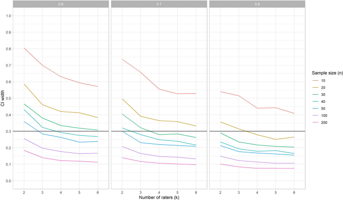
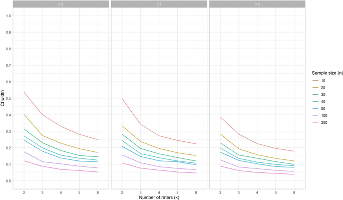
When no rater deviates, the 95% CI width around the ICC is the same for the different variances (v) and the different ICC methods (one-way, agreement or consistency). However, the correlation r does impact the width of the 95% CI: an increase of r leads to a decrease of the width (i.e., smaller confidence intervals) (Fig. 6). This means that when we expect the ICC to be 0.7 (i.e., we assume the measurements will be correlated with 0.7) the required sample size will be larger to obtain an ICC with the same precision than when we expect the ICC to be 0.8.
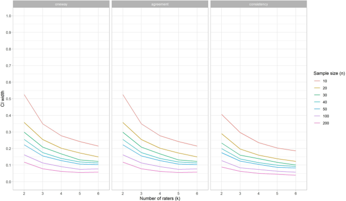
When one rater deviates, the width of the 95% CI does not change for the ICCconsistency, but it does increase for ICCagreement, and even more for ICCone-way (see Fig. 7).
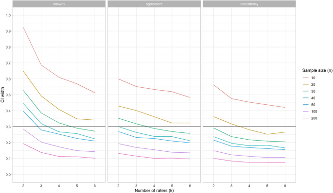
The 95% CI width around the ICC estimation for specific conditions can be used to determine what the optimal trade-off is for the sample size of patients and the number of repeated measures in these situations. In Fig. 6 (where we show results averaged over the three effects models) we can see that in the situation that no rater deviates, and v = 1, and we wish to estimate an ICC for three raters (k = 3), we need between 40 and 50 patients to obtain a CI width around the point estimation of 0.3 when r = 0.6 (i.e., + /– 0.15) (Fig. 6, left panel). If r is 0.7, then 30 patients is enough to reach the same precision (Fig. 6, middle panel), while if r = 0.8 20 patients is sufficient (Fig. 6, right panel). When one of the raters deviates, the chosen ICC method impacts the 95% CI width, in addition to the r (Fig. 7). To come to a 95% CI width of 0.3 around the point estimate when r = 0.8, v = 1, for a ICCagreement the sample size should be increased to 40, while the ICC one-way would require a sample size of 50.
The CI width for SEM estimation decreases when r increases (Fig. 8), similar as for ICC. However, in general, the width for SEM was smaller than for ICCs (Fig. 6).
When one rater deviates, the width of the 95% CI does not change for SEMconsistency, but it does increase for SEMagreement, and SEMone-way (see Fig. 9). In general, the width of the 95% CI is lower for SEM than it is for ICC. This means that in general, the SEM can be estimated with more precision than the ICC under the same conditions.
As shown in the results of our simulation study, sample size recommendations are dependent on the specific conditions of the study design at hand. Therefore, based on these simulation studies, we have created a Sample size decision assistant that is freely available as an online application to inform the choice about the sample size and number of repeated measurements in a reliability study.
The Sample size decision assistant shows the implications of decisions about the study design on the power of the study, by using any of the three procedures described in the methods section (i.e., the width of the confidence interval (CI width) procedure, the CI lower limit procedure, and the MSE ratio procedure). Each procedure requires some assumptions about the study design as input, as described in Table 3. When you choose to use either the CI lower limit procedure or the MSE ratio procedure, you are asked to indicate what the target design is. The target design is the intended sample size of patients or the number of repeated measurements (e.g., raters), decided upon at the start of the study. For the MSE ratio procedure you are also asked to indicate the adapted design, which refers to the number of patients or repeated measurements of the new design, e.g., the numbers that are included in the study so far. For both procedures you are asked to indicate the target width of the 95% CI of the parameter of interest. The width depends of the unit of measurements. As the range of the ICC is always between 0 and 1, the range of the target width is fixed, and it is set default at 0.3 in the online application. However, the SEM depends on the unit of measurement, and changes across conditions v. Therefore, in the online application, the range for the target width of the 95% CI for the SEM changes across conditions v, and various default settings are used.
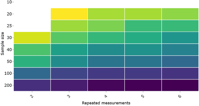
By scrolling over the different blocks in the online application, we can easily see what the consequence is for the width of the CI around the estimated ICC when adding an extra rater or including more patients. For example, when we use 3 raters and 20 patients, the estimated width of the CI around the ICC estimation is 0.293; or when k = 2 and n = 30 the width of te CI is 0.278; and when k = 2 and n = 25 the width is 0.33. In the online application this information automatically pops up.
If we compare the results for various conditions in the application, we see that the impact of whether or not a systematic difference exist on the sample size recommendations is much larger than the impact of different values for the variance between the scores, specifically when in the one-way random effects model, or the two-way random effects model for agreement.
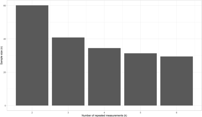
The second procedure that can be used in the design phase is the CI lower limit procedure. This procedure is developed by Zou for ICCone-way. Note that procedure may lead to an overestimation of the required sample size for ICCs based on a two-way effects model (see results, and (Donner and Eliasziw 1987)). An example to use this procedure: if we expect the ICC to be 0.8, and we accept a lower CI limit of the ICC of 0.65, depending on the number of repeated measurements that will be collected, the adequate sample size is given (see Fig. 11). For example, for k = 3, a sample size of 40 is appropriate (under the given conditions). As this procedure is based on a formula, it can be used beyond the conditions chosen in the simulated data.
The third procedure, the MSE ratio procedure, is most suitable when we have started the data collection and realize that the target design cannot be reached. In that case we want to know how an adapted design compares to our target design that was described in the study protocol. Suppose that patients were observed in clinical practice and scored by three raters (k = 3) at (about) the same time. We envisioned 50 patients (i.e., target design). The number of raters cannot be changed anymore, as patients will possibly have changed on the construct measured, or it is logistically impossible to invite the same patients to come back for another measurement. Based on the results of previous studies, or by running preliminary analyses on the collected data within this study, we can make assumptions about: the expected correlation between the raters (i.e., the repeated measurements; e.g., 0.8), whether we expect one of these raters to systematically deviate from the others (e.g., no), and the expected variance in score (e.g., 10). Suppose we have collected data of three raters that each measured 25 patients; this is our adapted design. Now, we can see how much the 95% CI will increase, when we don’t continue collecting data until we have included 50 patients (i.e., your target design) (Fig. 12). The 95% CI will increase approximately from 0.2 that we would have had if we measured 50 patients three times (i.e., target design) to 0.3 now in the adapted design.
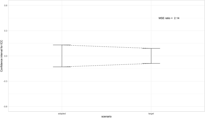
Another way to use this method, is to see how much one of the two variables n or k should increase to preserve the same level of precision as in the target design. For example, in the target design 3 raters would assess 25 patients. As one of the raters dropped out, there are only 2 raters in the adapted design. The MSE ratio in this scenario was 1.43. To achieve the same level of precision in the adapted design with 2 raters as in the target design (n = 25, k = 3), the sample size should be increased by 1.43, resulting in a sample size of n = 36.
From the simulation studies we learn that most gain in precision (i.e., largest change in MSE values) can be obtained by increasing an initially small sample sizes or small number of repeated measures. For example, an increase from 2 to 3 raters gains more precision than from 4 to 5 raters, or when the sample size is increased from 10 to 20 compared to an increase from 40 to 50. Moreover, results show that the expected ICC (i.e., correlation between the repeated measurements), and the presence of a systematic difference have most influence on the precision of the ICC and SEM estimations. Specifically, when the correlation increases the precision increases (i.e., smaller MSE values, and smaller width of CI). When one rater deviates the MSE values for ICCone-way, SEMone-way/SEMagreement increase, the coverage of the ICCagreement and the ICCone-way changes and the width of the CI increases for the ICCone-way and ICCagreement, but not for the ICCconsistency. For example, to achieve an estimation with a width of the confidence interval of approximately 0.3 using an ICCagreement model when one of the three raters systematically deviates, the sample size needs to be around 40 (when r = 0.7) or 30 (when r = 0.8). When no systematic difference occurs between the three repeated measurements, the required sample size when r = 0.7 or r = 0.8, can be lowered to approximately n = 35 or n = 20, respectively, to obtain an estimation of the ICCagreement with a CI width of 0.3.
Throughout this paper, we used ‘raters’ as the source of variation that varied across the repeated measurements, but the results are not limited to the use of raters as the source of variation. Accordingly, all results and recommendations also hold for other sources of variation, however feasibility of the recommendations may differ. For example, in a test–retest reliability study ‘occasion’ is the sources of variation of interest. However, it may not be feasible to have three repeated measurements of patients as patients may not be stable between three measurements. When only two repeated measurements can be obtained, sample size requirements increase. Note, that we only took one-way or two-way effect models into account, and we cannot generalize these results to three-way effects models. We did not simulate conditions of n between 50 and 100. Therefore, we can only roughly recommend that when there is a systematic difference between the repeated measurements, required sample size will increase up to 100, specifically when the ICCone-way model is used, and likely around 75 when the ICCagreement is used. Recommendations for specific conditions can be found in the online application (https://iriseekhout.shinyapps.io/ICCpower/).
The selected sample of patients should be representative of the population in which the instrument will be used, as the variation of the patients will influence the ICC value. The result of the study can only be generalized to this population. The same holds for the selection of professionals that are involved in the measurements and any other source of variation that is being varied across the repeated measurements. Selecting only well trained raters in a reliability study will possibly decrease the variation between the raters, and subsequently influence the ICC and SEM estimation. Therefore, it is important to well-consider which patients and which professionals and other sources of variation are selected for the study. For an appropriate interpretation of the ICC and SEM values, complete reporting of research questions and rationale of choices made in the design (i.e., choice in type and number of patients, raters, equipment, circumstances etc.) is indispensable (Mokkink et al. 2022).
As measurements can be expensive and burdensome to patients and professionals, we do not recommend to collect more data than required to estimate ICC or SEM values as this would lead to research waste. Therefore, it is important to involve these feasibility aspects in the decisions of the optimal sample size and repeated measurements. When a systematic difference between raters occurs, we showed that the use of a one-way model requires a higher sample size compared to two-way random effect models for agreement, which subsequently requires a higher sample size than the two-way mixed model for consistency (see Fig. 7). The difference in data collection between the models, is that two-way effect models require extra predefined measurement conditions (Mokkink et al. 2022), e.g., only rater A and B are involved and measure all patients, while in one-way effects models no measurement conditions are defined, and any rater could measure the patient at any occasion. As the goal of a reliability study is often to understand the influence of a specific source of variation (e.g., the rater) on the score (i.e., its systematic difference), a two-way random effects model is often the preferred statistical method (Mokkink et al. 2022). We have showed that this is also the most efficient model precision-wise.
Our recommendations are in line with other recommendations. Previous studies showed that the sample size is dependent on the correlation between the repeated measurements (Shoukri et al. 2004), and that adding more than three repeated measurements gains only little precision (Giraudeau and Mary 2001; Shoukri et al. 2004). However, we provide recommendations under more conditions, i.e., for three types of effect models, and with and without systematic differences. Moreover, we present our recommendations in a user-friendly way by the development of the Sample size decision assistant, that is available in the online application.
As an example, we used an appropriate width of the confidence interval around the point estimate of 0.3. We could have chosen another width. Zou (2012) used 0.2 as an appropriate interval, which we considered quite small. However, in the online application the consequences on precision with a width of 0.2 can be examined as well.
In this study we considered a large variety of conditions for the variables n, k, v, r. In contrast to previous studies on required sample sizes, we used three different and commonly used statistical models to estimate the parameters, and incorporated systematic differences between the repeated measurements. Moreover, we investigated the bias and precision of the ICC as well as of the SEM.
Generally, we can see that the SEM can be estimated with more precision than the ICC. When in doubt, we propose to use recommendations on sample size and number of repeated measurements for ICC.
Furthermore, as conclusion based on simulation studies are restricted to the conditions investigated, our study is limited in that aspect. We only simulated three conditions of the correlations between repeated measurements (r = 0.6, 0.7 and 0.8) and we concluded that the presence of a systematic difference has most influence on the width of the confidence interval, specifically with the larger correlations (0.7 and 0.8). As we did not simulate the condition 0.9, we don’t know to what extent that holds for this condition. Moreover, we did not simulate any condition for n between 50 and 100. Therefore, we cannot give precise recommendations for when k = 2, as it is likely that the appropriate sample size in this situation will be between 50 and 100. Last, we simulated a systematic difference in one (k = 2–6) or two (k = 2–4) raters. However, the way the two raters deviated in the latter condition was the same (i.e., by increasing the average score of the rater with 1 standard deviation in score). Other ways that raters may deviate were not investigated. Nevertheless, we feel that the use of one standard deviation deviance for one or two raters demonstrates a sufficient difference to test the relative performance of the two-way effect models, but not too large to be unrealistic.
We used multilevel methods to estimate the variance components that are subsequently used to calculate ICCs and SEMs. These methods are robust against missing data and able to deal with unbalanced designs. However, investigating the impact of missing data on the precision of the ICC and SEM estimations was beyond the scope of this study.
Our findings are utilized in an online application. The different ways in which this tool can be used provides insight into the influence of various conditions on the sample sizes and into the trade-off between various choices. Using this tool enables researchers to use the study findings to estimate required sample sizes for number of patients or number of raters (or other repetitions) for an efficient design of reliability studies. We aim to continue to improve the design and layout of the app to improve usability and user-friendliness of the application and to broaden the scope of the recommendations to match with the demands of users.
The syntax used to generate the datasets that were analyzed during the current study is available in “Appendix 1”.
This work is part of the research programme Veni (recieved by LM) with Grand No. 91617098 funded by ZonMw (The Netherlands Organisation for Health Research and Development). The funding body has no role in the study design, the collection, analysis, and interpretation of data or in the writing of this manuscript.
